R-kieli

Last time updated: **2021-06-22 21:06:02**

1 Install.packages

To get started install at least these: r-paketit.txt

PACKAGES <- scan(url("http://muuankarski.kapsi.fi/luntti/r-paketit.txt"), what="character")
inst <- match(PACKAGES, .packages(all=TRUE))
need <- which(is.na(inst))
if (length(need) > 0) install.packages(PACKAGES[need], Ncpus = 4)
# Or one liner
PACKAGES <- scan(url("http://muuankarski.kapsi.fi/luntti/r-paketit.txt"), what="character"); inst <- match(PACKAGES, .packages(all=TRUE)); install.packages(PACKAGES[which(is.na(inst))])

update.packages(checkBuilt = TRUE, ask = FALSE, Ncpus = parallel::detectCores())

# jos systeemikirjastoon niin sudo su ...

# paketit github:sta
PACKAGES <- scan(url("http://muuankarski.kapsi.fi/luntti/r_paketit_github.txt"), what="character")
for (pkg in PACKAGES) devtools::install_github(pkg)

# paketit gitlab:sta
PACKAGES <- scan(url("http://muuankarski.kapsi.fi/luntti/r_paketit_gitlab.txt"), what="character")
for (pkg in PACKAGES) devtools::install_gitlab(pkg)

2 Rivitä stringit

# character
x$y <- gsub('(.{1,30})(\\s|$)', '\\1\n', x$y)
# faktori
levels(x$y) <- gsub('(.{1,30})(\\s|$)', '\\1\n', levels(x$y))

3 Data manipulation

• tidyr & dplyr cheatsheet
• Garrett Grolemund - Data Wrangling with R slaidit

3.1 Create the data sets

library(tidyr)
library(dplyr)
# cases
df <- data.frame(country = c("FR", "DE", "US", "FR", "DE", "US", "FR", "DE", "US"),
                 year = c(2011,2011,2011,2012,2012,2012,2013,2013,2013),
                 n = c(7000,5800,15000,6900,6000,14000,7000,6200,13000),
                 stringsAsFactors = FALSE)
cases <- spread(df, year, n)
#                      
df <- data.frame(city = c("New York", "New York", "London", "London", "Beijing", "Beijing"),
                 size = c("large", "small", "large", "small", "large", "small"),
                 amount = c(23,14,22,16,121,56),
                 stringsAsFactors = FALSE)
pollution <- df
# storms
storms <- data.frame(storm = c("Alberto", "Alex", "Allison", "Ana", "Arlene", "Arthur"),
                     wind = c(110,45,65,40,50,45),
                     pressure = c(1007,1009,1005,1013,1010,1010),
                     date = as.Date(c("2000-08-03", "1998-07-27", "1995-06-03", "1997-06-30", "1999-06-11", "1996-06-17")),
                     stringsAsFactors = FALSE)
# songs
songs <- data.frame(song = c("Across the Universe", "Come Together", "Hello, Goodbye", "Peggy Sue"),
                    name = c("John", "John", "Paul", "Buddy"),
                    stringsAsFactors = FALSE)
# artists
artists <- data.frame(name = c("George", "John", "Paul", "Ringo"),
                      plays = c("sitar", "guitar", "bass", "drums"),
                      stringsAsFactors = FALSE)

3.2 tidyr

cases

##   country  2011  2012  2013
## 1      DE  5800  6000  6200
## 2      FR  7000  6900  7000
## 3      US 15000 14000 13000

gather(cases, # data
       "year", # name of the key variable
       "n", # name of valut var
       2:4) # variables NOT tidy

##   country year     n
## 1      DE 2011  5800
## 2      FR 2011  7000
## 3      US 2011 15000
## 4      DE 2012  6000
## 5      FR 2012  6900
## 6      US 2012 14000
## 7      DE 2013  6200
## 8      FR 2013  7000
## 9      US 2013 13000

pollution

##       city  size amount
## 1 New York large     23
## 2 New York small     14
## 3   London large     22
## 4   London small     16
## 5  Beijing large    121
## 6  Beijing small     56

spread(pollution, # data
       size, # class-var
       amount) # amount

##       city large small
## 1  Beijing   121    56
## 2   London    22    16
## 3 New York    23    14

storms

##     storm wind pressure       date
## 1 Alberto  110     1007 2000-08-03
## 2    Alex   45     1009 1998-07-27
## 3 Allison   65     1005 1995-06-03
## 4     Ana   40     1013 1997-06-30
## 5  Arlene   50     1010 1999-06-11
## 6  Arthur   45     1010 1996-06-17

storms2 <- separate(storms, date, c("year", "month", "day"), sep = "-")
storms2

##     storm wind pressure year month day
## 1 Alberto  110     1007 2000    08  03
## 2    Alex   45     1009 1998    07  27
## 3 Allison   65     1005 1995    06  03
## 4     Ana   40     1013 1997    06  30
## 5  Arlene   50     1010 1999    06  11
## 6  Arthur   45     1010 1996    06  17

unite(storms2, "date", year, month, day, sep = "-")

##     storm wind pressure       date
## 1 Alberto  110     1007 2000-08-03
## 2    Alex   45     1009 1998-07-27
## 3 Allison   65     1005 1995-06-03
## 4     Ana   40     1013 1997-06-30
## 5  Arlene   50     1010 1999-06-11
## 6  Arthur   45     1010 1996-06-17

3.3 dplyr

library(dplyr)
library(ggplot2)
tbl_df(diamonds)

## # A tibble: 53,940 x 10
##    carat cut       color clarity depth table price     x     y     z
##    <dbl> <ord>     <ord> <ord>   <dbl> <dbl> <int> <dbl> <dbl> <dbl>
##  1  0.23 Ideal     E     SI2      61.5    55   326  3.95  3.98  2.43
##  2  0.21 Premium   E     SI1      59.8    61   326  3.89  3.84  2.31
##  3  0.23 Good      E     VS1      56.9    65   327  4.05  4.07  2.31
##  4  0.29 Premium   I     VS2      62.4    58   334  4.2   4.23  2.63
##  5  0.31 Good      J     SI2      63.3    58   335  4.34  4.35  2.75
##  6  0.24 Very Good J     VVS2     62.8    57   336  3.94  3.96  2.48
##  7  0.24 Very Good I     VVS1     62.3    57   336  3.95  3.98  2.47
##  8  0.26 Very Good H     SI1      61.9    55   337  4.07  4.11  2.53
##  9  0.22 Fair      E     VS2      65.1    61   337  3.87  3.78  2.49
## 10  0.23 Very Good H     VS1      59.4    61   338  4     4.05  2.39
## # … with 53,930 more rows

diamonds$x %>%
  mean() %>%
  round(2)

## [1] 5.73

3.3.1 select() - subset rows

storms
# drop vars
select(storms, -storm)
# subset rows
filter(storms, wind >= 50)
# subset rows - multiple conditions
filter(storms,
       wind >= 50,
       storm %in% c("Alberto", "Alex", "Allison"))

3.3.1.1 More select-commands

- # Select everything but
  : # Select range
  contains() # Select columns whose name contains a character string
ends_with() # Select columns whose name ends with a string
everything() # Select every column
matches() # Select columns whose name matches a regular expression
num_range() # Select columns named x1, x2, x3, x4, x5
one_of() # Select columns whose names are in a group of names
starts_with() # Select columns whose name starts with a character string

3.3.2 mutate () - create new vars

mutate(storms, ratio = pressure / wind)

##     storm wind pressure       date     ratio
## 1 Alberto  110     1007 2000-08-03  9.154545
## 2    Alex   45     1009 1998-07-27 22.422222
## 3 Allison   65     1005 1995-06-03 15.461538
## 4     Ana   40     1013 1997-06-30 25.325000
## 5  Arlene   50     1010 1999-06-11 20.200000
## 6  Arthur   45     1010 1996-06-17 22.444444

mutate(storms,ratio = pressure / wind,
       inverse = ratio^-1)

##     storm wind pressure       date     ratio    inverse
## 1 Alberto  110     1007 2000-08-03  9.154545 0.10923535
## 2    Alex   45     1009 1998-07-27 22.422222 0.04459861
## 3 Allison   65     1005 1995-06-03 15.461538 0.06467662
## 4     Ana   40     1013 1997-06-30 25.325000 0.03948667
## 5  Arlene   50     1010 1999-06-11 20.200000 0.04950495
## 6  Arthur   45     1010 1996-06-17 22.444444 0.04455446

3.3.2.1 More mutate fuctions

All take a vector of values and return a vector of values

pmin(), pmax() # Element-wise min and max
cummin(), cummax() # Cumulative min and max
cumsum(), cumprod() # Cumulative sum and product
between() # Are values between a and b?
cume_dist() # Cumulative distribution of values
cumall(), cumany() # Cumulative all and any
cummean() # Cumulative mean
lead(), lag() # Copy with values one position
ntile() #Bin vector into n buckets
dense_rank(), min_rank(), percent_rank(), row_number() # Various ranking methods

3.3.3 summarise() - Change unit

pollution %>% 
  summarise(median = median(amount), 
            variance = var(amount))

##   median variance
## 1   22.5   1731.6

3.3.3.1 Good summary functions

All take a vector of values and return a single value

min(), max() # Minimum and maximum values
mean() # Mean value
median() # Median value
sum() # Sum of values
var, sd() # Variance and standard deviation of a vector
first() # First value in a vector
last() # Last value in a vector
nth() # Nth value in a vector
n() # The number of values in a vector
n_distinct() # The number of distinct values in a vector

3.3.4 Grouped analysis

h <- pollution %>% group_by(city)
h

## # A tibble: 6 x 3
## # Groups:   city [3]
##   city     size  amount
##   <chr>    <chr>  <dbl>
## 1 New York large     23
## 2 New York small     14
## 3 London   large     22
## 4 London   small     16
## 5 Beijing  large    121
## 6 Beijing  small     56

ungroup(h)

## # A tibble: 6 x 3
##   city     size  amount
##   <chr>    <chr>  <dbl>
## 1 New York large     23
## 2 New York small     14
## 3 London   large     22
## 4 London   small     16
## 5 Beijing  large    121
## 6 Beijing  small     56

pollution

##       city  size amount
## 1 New York large     23
## 2 New York small     14
## 3   London large     22
## 4   London small     16
## 5  Beijing large    121
## 6  Beijing small     56

pollution  %>% group_by(city) %>%
  summarise(mean = mean(amount),
            sum = sum(amount),
            n = n())

## # A tibble: 3 x 4
##   city      mean   sum     n
##   <chr>    <dbl> <dbl> <int>
## 1 Beijing   88.5   177     2
## 2 London    19      38     2
## 3 New York  18.5    37     2

pollution %>% 
  group_by(city) %>% 
  summarise(mean = mean(amount), sum = sum(amount), n = n())

## # A tibble: 3 x 4
##   city      mean   sum     n
##   <chr>    <dbl> <dbl> <int>
## 1 Beijing   88.5   177     2
## 2 London    19      38     2
## 3 New York  18.5    37     2

# data(tb)
# tb %>% 
#   group_by(country, year) %>% 
#   summarise(cases = sum(cases)) %>% 
#   summarise(cases = sum(cases))

Error in FUN(X[[1L]], ...) : 
  only defined on a data frame with all numeric variable

3.3.5 Rank groups

rank by which “cylinder group” highest total hp. (makes no sense, but was useful)

library(dplyr)
mtcars %>% 
  slice(1:10) %>% 
  dplyr::select(cyl,hp) %>% 
  group_by(cyl) %>% 
  mutate(sum_hp = sum(hp, na.rm = TRUE)) %>% 
  ungroup() %>% 
  arrange(sum_hp) %>% 
  mutate(rank = dense_rank(sum_hp))

## # A tibble: 10 x 4
##      cyl    hp sum_hp  rank
##    <dbl> <dbl>  <dbl> <int>
##  1     4    93    250     1
##  2     4    62    250     1
##  3     4    95    250     1
##  4     8   175    420     2
##  5     8   245    420     2
##  6     6   110    558     3
##  7     6   110    558     3
##  8     6   110    558     3
##  9     6   105    558     3
## 10     6   123    558     3

3.3.6 Järjestä data

arrange(storms, wind)

##     storm wind pressure       date
## 1     Ana   40     1013 1997-06-30
## 2    Alex   45     1009 1998-07-27
## 3  Arthur   45     1010 1996-06-17
## 4  Arlene   50     1010 1999-06-11
## 5 Allison   65     1005 1995-06-03
## 6 Alberto  110     1007 2000-08-03

arrange(storms, -wind)

##     storm wind pressure       date
## 1 Alberto  110     1007 2000-08-03
## 2 Allison   65     1005 1995-06-03
## 3  Arlene   50     1010 1999-06-11
## 4    Alex   45     1009 1998-07-27
## 5  Arthur   45     1010 1996-06-17
## 6     Ana   40     1013 1997-06-30

arrange(storms, desc(wind), desc(date))

##     storm wind pressure       date
## 1 Alberto  110     1007 2000-08-03
## 2 Allison   65     1005 1995-06-03
## 3  Arlene   50     1010 1999-06-11
## 4    Alex   45     1009 1998-07-27
## 5  Arthur   45     1010 1996-06-17
## 6     Ana   40     1013 1997-06-30

3.3.7 the pipe operatos

storms %>% 
  filter(wind >= 50) %>% 
  dplyr::select(storm, pressure)

##     storm pressure
## 1 Alberto     1007
## 2 Allison     1005
## 3  Arlene     1010

pollution  %>% group_by(city) %>%
  summarise(mean = mean(amount),
            sum = sum(amount),
            n = n())

## # A tibble: 3 x 4
##   city      mean   sum     n
##   <chr>    <dbl> <dbl> <int>
## 1 Beijing   88.5   177     2
## 2 London    19      38     2
## 3 New York  18.5    37     2

storms %>% 
  mutate(ratio = pressure / wind) %>%
  dplyr::select(storm, ratio)

##     storm     ratio
## 1 Alberto  9.154545
## 2    Alex 22.422222
## 3 Allison 15.461538
## 4     Ana 25.325000
## 5  Arlene 20.200000
## 6  Arthur 22.444444

pollution  %>% group_by(city) %>%
  mutate(mean = mean(amount),
         sum = sum(amount),
         n = n())

## # A tibble: 6 x 6
## # Groups:   city [3]
##   city     size  amount  mean   sum     n
##   <chr>    <chr>  <dbl> <dbl> <dbl> <int>
## 1 New York large     23  18.5    37     2
## 2 New York small     14  18.5    37     2
## 3 London   large     22  19      38     2
## 4 London   small     16  19      38     2
## 5 Beijing  large    121  88.5   177     2
## 6 Beijing  small     56  88.5   177     2

3.3.8 join() - merging data.frames

library(dplyr)

songs

##                  song  name
## 1 Across the Universe  John
## 2       Come Together  John
## 3      Hello, Goodbye  Paul
## 4           Peggy Sue Buddy

artists

##     name  plays
## 1 George  sitar
## 2   John guitar
## 3   Paul   bass
## 4  Ringo  drums

left_join(songs, artists, by = "name")

##                  song  name  plays
## 1 Across the Universe  John guitar
## 2       Come Together  John guitar
## 3      Hello, Goodbye  Paul   bass
## 4           Peggy Sue Buddy   <NA>

inner_join(songs, artists, by = "name")

##                  song name  plays
## 1 Across the Universe John guitar
## 2       Come Together John guitar
## 3      Hello, Goodbye Paul   bass

#outer_join(songs, artists, by = "name")

semi_join(songs, artists, by = "name")

##                  song name
## 1 Across the Universe John
## 2       Come Together John
## 3      Hello, Goodbye Paul

anti_join(songs, artists, by = "name")

##        song  name
## 1 Peggy Sue Buddy

dplyr::bind_cols(x,y)
dplyr::bind_rows
dplyr::union
dplyr::intersect
dplyr::setdif

3.4 Base-R

3.4.1 Na solujen poistaminen

# yksi muuttuja
df <- df[!is.na(df$Var1),]
# kaikki rivit joilla na
df2 <- na.omit(df) 

3.4.2 Faktorit numeerisiksi

d <- storms
d$f <- as.character(d$wind)
d

##     storm wind pressure       date   f
## 1 Alberto  110     1007 2000-08-03 110
## 2    Alex   45     1009 1998-07-27  45
## 3 Allison   65     1005 1995-06-03  65
## 4     Ana   40     1013 1997-06-30  40
## 5  Arlene   50     1010 1999-06-11  50
## 6  Arthur   45     1010 1996-06-17  45

mean(d$f)

## [1] NA

d$f <- factor(d$f)
d$f <- as.numeric(levels(d$f))[d$f]

mean(d$f)

## [1] 59.16667

# Or 

d$f <- as.integer(d$f)
mean(d$f)

## [1] 59.16667

3.4.3 Removing duplicats

d <- rbind(storms,storms)
d

##      storm wind pressure       date
## 1  Alberto  110     1007 2000-08-03
## 2     Alex   45     1009 1998-07-27
## 3  Allison   65     1005 1995-06-03
## 4      Ana   40     1013 1997-06-30
## 5   Arlene   50     1010 1999-06-11
## 6   Arthur   45     1010 1996-06-17
## 7  Alberto  110     1007 2000-08-03
## 8     Alex   45     1009 1998-07-27
## 9  Allison   65     1005 1995-06-03
## 10     Ana   40     1013 1997-06-30
## 11  Arlene   50     1010 1999-06-11
## 12  Arthur   45     1010 1996-06-17

d[!duplicated(d[c("storm","wind","pressure")]),]

##     storm wind pressure       date
## 1 Alberto  110     1007 2000-08-03
## 2    Alex   45     1009 1998-07-27
## 3 Allison   65     1005 1995-06-03
## 4     Ana   40     1013 1997-06-30
## 5  Arlene   50     1010 1999-06-11
## 6  Arthur   45     1010 1996-06-17

3.4.4 Renaming variables

# built-in
names(d)[names(d)=="storm"] <- "newName"
d

##    newName wind pressure       date
## 1  Alberto  110     1007 2000-08-03
## 2     Alex   45     1009 1998-07-27
## 3  Allison   65     1005 1995-06-03
## 4      Ana   40     1013 1997-06-30
## 5   Arlene   50     1010 1999-06-11
## 6   Arthur   45     1010 1996-06-17
## 7  Alberto  110     1007 2000-08-03
## 8     Alex   45     1009 1998-07-27
## 9  Allison   65     1005 1995-06-03
## 10     Ana   40     1013 1997-06-30
## 11  Arlene   50     1010 1999-06-11
## 12  Arthur   45     1010 1996-06-17

# using plyr
plyr::rename(d, c("wind"="newName2", "pressure"="newName3"))

##    newName newName2 newName3       date
## 1  Alberto      110     1007 2000-08-03
## 2     Alex       45     1009 1998-07-27
## 3  Allison       65     1005 1995-06-03
## 4      Ana       40     1013 1997-06-30
## 5   Arlene       50     1010 1999-06-11
## 6   Arthur       45     1010 1996-06-17
## 7  Alberto      110     1007 2000-08-03
## 8     Alex       45     1009 1998-07-27
## 9  Allison       65     1005 1995-06-03
## 10     Ana       40     1013 1997-06-30
## 11  Arlene       50     1010 1999-06-11
## 12  Arthur       45     1010 1996-06-17

# using dplyr
dplyr::rename(d, newName2=wind, newName3=pressure)

##    newName newName2 newName3       date
## 1  Alberto      110     1007 2000-08-03
## 2     Alex       45     1009 1998-07-27
## 3  Allison       65     1005 1995-06-03
## 4      Ana       40     1013 1997-06-30
## 5   Arlene       50     1010 1999-06-11
## 6   Arthur       45     1010 1996-06-17
## 7  Alberto      110     1007 2000-08-03
## 8     Alex       45     1009 1998-07-27
## 9  Allison       65     1005 1995-06-03
## 10     Ana       40     1013 1997-06-30
## 11  Arlene       50     1010 1999-06-11
## 12  Arthur       45     1010 1996-06-17

3.4.5 Rename factor levels

# built-in
levels(x)[levels(x)=="one"] <- "uno"
levels(x)[3] <- "three"
levels(x) <- c("one","two","three")

# plyr
library(plyr)
revalue(x, c("beta"="two", "gamma"="three"))
mapvalues(x, from = c("beta", "gamma"), to = c("two", "three"))

3.4.6 Subset data

# based on regexpr in string
d[ with(d, grepl("Ar", newName)),]

##    newName wind pressure       date
## 5   Arlene   50     1010 1999-06-11
## 6   Arthur   45     1010 1996-06-17
## 11  Arlene   50     1010 1999-06-11
## 12  Arthur   45     1010 1996-06-17

# subset string
s <- d$newName
s[grepl("Ar",s)]

## [1] "Arlene" "Arthur" "Arlene" "Arthur"

3.4.7 Remove objects from workspace

# Remove all objects but
rm(list=setdiff(ls(), c("x","y")))
# Remove all
rm(list=ls(all=TRUE)) 
# Remove a list
rm(list = c('x','y'))
## or
rm(x,y)

source

3.4.8 Järjestä data

d <- storms
# 
d[order(d$wind),]

##     storm wind pressure       date
## 4     Ana   40     1013 1997-06-30
## 2    Alex   45     1009 1998-07-27
## 6  Arthur   45     1010 1996-06-17
## 5  Arlene   50     1010 1999-06-11
## 3 Allison   65     1005 1995-06-03
## 1 Alberto  110     1007 2000-08-03

# tai with ja useampi muuttuja
d[with(d, order(wind, -pressure)), ]

##     storm wind pressure       date
## 4     Ana   40     1013 1997-06-30
## 6  Arthur   45     1010 1996-06-17
## 2    Alex   45     1009 1998-07-27
## 5  Arlene   50     1010 1999-06-11
## 3 Allison   65     1005 1995-06-03
## 1 Alberto  110     1007 2000-08-03

# fatorilevelit jatkuvan muuttujan mukaan (order) 
factor(d$storm, levels=d[order(d$pressure),]$storm)

## [1] Alberto Alex    Allison Ana     Arlene  Arthur 
## Levels: Allison Alberto Alex Arlene Arthur Ana

Tulosta pilkulla erotettu vektori

vector <- c("one","two","three")
cat(paste(shQuote(vector, type="cmd"), collapse=", "))

## "one", "two", "three"

vector <- c(1,2,3)
cat(paste(vector, collapse=","))

## 1,2,3

3.5 links

• tidy data and tidy tools
• Lists and data cleaning
• Hadley Wickham on regular expressions

---

---

4 Ordering bar plots in ggplot2

4.1 Data

fruits <- c(rep("apples",4), rep("oranges",4), rep("pears",4),rep("bananas",4))
basket <- rep(c("basket1","basket2","basket3","basket4"),4)
value <- c(10,15,20,25,
           25,15,20,15,
           50,40,30,20,
           15,30,30,40)

df <- data.frame(basket,value,fruits, stringsAsFactors = FALSE)

fill_palette <- c("#FF0000", # red for apple
                  "#FF9900", # orange for orange
                  "#66FF33", # green for pears
                  "#FFFF00" # yellow for bananas
)

head(df)

##    basket value  fruits
## 1 basket1    10  apples
## 2 basket2    15  apples
## 3 basket3    20  apples
## 4 basket4    25  apples
## 5 basket1    25 oranges
## 6 basket2    15 oranges

str(df)

## 'data.frame':    16 obs. of  3 variables:
##  $ basket: chr  "basket1" "basket2" "basket3" "basket4" ...
##  $ value : num  10 15 20 25 25 15 20 15 50 40 ...
##  $ fruits: chr  "apples" "apples" "apples" "apples" ...

4.2 Plots

4.2.1 Without any ordering

• bars are ordered alphabetically by name
• fills are ordered alphabetically by name

library(ggplot2)
ggplot(data=df, 
       aes(x=basket,
           y=value,
           fill=fruits)) +
  geom_bar(stat="identity", 
           position = "stack") +
  scale_fill_manual(values=fill_palette)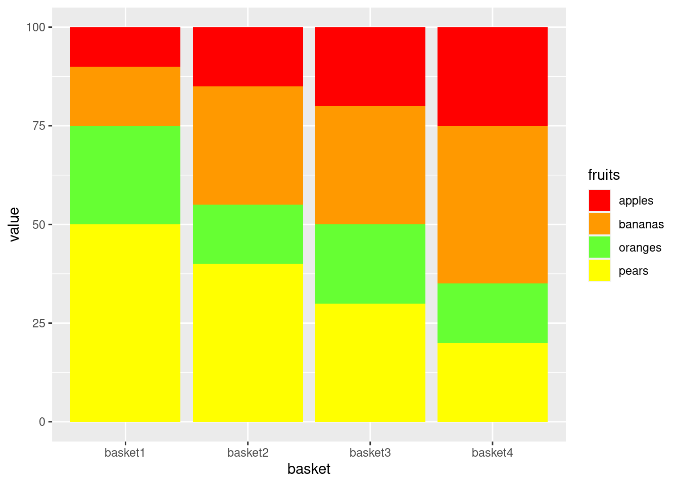

4.2.2 Manual ordering

4.2.2.1 Manual order the bars

library(ggplot2)
df$basket <- factor(df$basket, levels=c("basket2","basket3","basket1","basket4"))

ggplot(data=df, 
       aes(x=basket,
           y=value,
           fill=fruits)) +
  geom_bar(stat="identity", 
           position = "stack") +
  scale_fill_manual(values=fill_palette)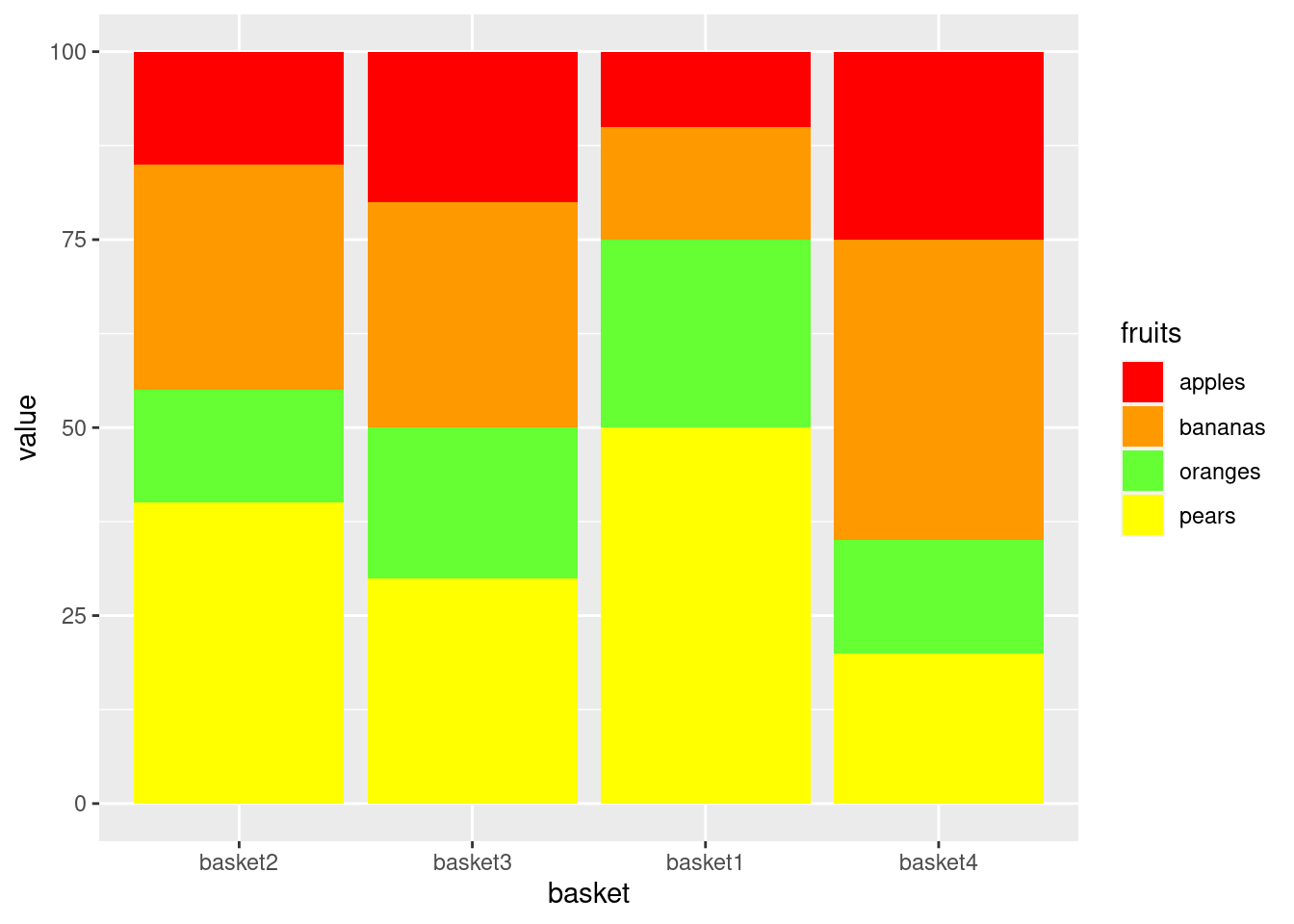

4.2.2.2 Manually match the fills with the fruits

Just manually order the factor levels to match the order of colors in fill_palette

library(ggplot2)
df$basket <- as.character(df$basket) # resetting the bar ordering
df$fruits <- factor(df$fruits, c("apples","oranges","pears","bananas"))

ggplot(data=df, 
       aes(x=basket,
           y=value,
           fill=fruits)) +
  geom_bar(stat="identity", 
           position = "stack") +
  scale_fill_manual(values=fill_palette)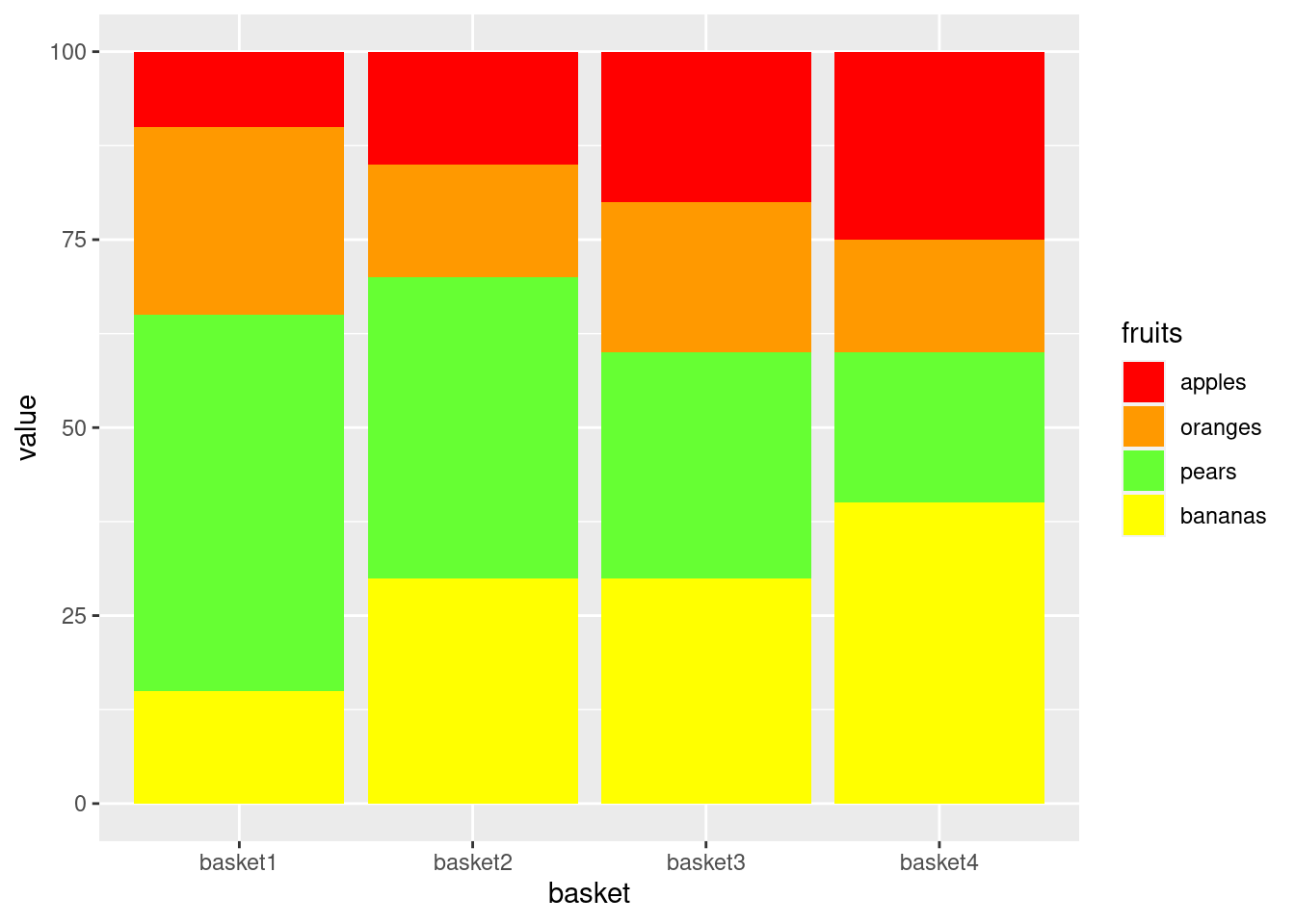

4.2.2.3 Reorder the legend to match the order of the fill

library(ggplot2)
df$fruits <- factor(df$fruits, c("apples","oranges","pears","bananas"))

ggplot(data=df, 
       aes(x=basket,
           y=value,
           fill=fruits)) +
  geom_bar(stat="identity", 
           position = "stack") +
  scale_fill_manual(values=fill_palette, 
                    guide = guide_legend(reverse=TRUE))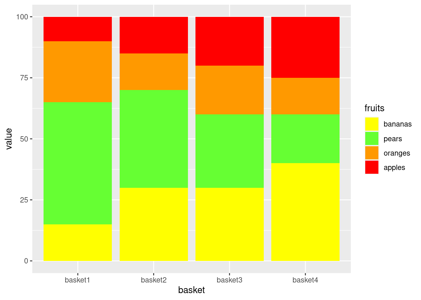

4.2.2.4 Reorder the fills manually

2.0 version of ggplot2 was introduced in late 2015 and orderaesthetics was depracated.

The new approach is to order the dataset by the grouping variable you want to order by as described in the 2nd or newest answer for this question: http://stackoverflow.com/questions/15251816/how-do-you-order-the-fill-colours-within-ggplot2-geom-bar

the old order way

library(ggplot2)
df$fruits <- factor(df$fruits, c("bananas","pears","oranges","apples"))

ggplot(data=df, 
       aes(x=basket,
           y=value,
           fill=fruits,
           order=fruits)) + # This WAS important!!
  geom_bar(stat="identity", 
           position = "stack") +
  scale_fill_manual(values=fill_palette, 
                    guide = guide_legend(reverse=TRUE))

With dplyr

library(ggplot2)
df$fruits <- factor(df$fruits, c("bananas","pears","oranges","apples"))

library(dplyr)
ggplot(data=dplyr::arrange(df,fruits), 
       aes(x=basket,
           y=value,
           fill=fruits)) + 
  geom_bar(stat="identity", 
           position = "stack") +
  scale_fill_manual(values=fill_palette, 
                    guide = guide_legend(reverse=TRUE))

With base R

library(ggplot2)
df$fruits <- factor(df$fruits, c("bananas","pears","oranges","apples"))

ggplot(data=df[order(df$fruits),], 
       aes(x=basket,
           y=value,
           fill=fruits)) + 
  geom_bar(stat="identity", 
           position = "stack") +
  scale_fill_manual(values=fill_palette, 
                    guide = guide_legend(reverse=TRUE))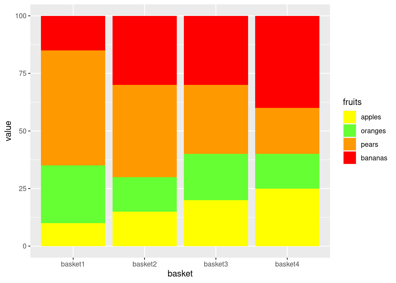

4.2.3 Automatic reordering

4.2.3.1 Order bars according to pears share

library(ggplot2)
df$basket <- factor(df$basket, 
                    levels=df[order(df[df$fruits == "pears",]$value),]$basket)

ggplot(data=df[order(df$fruits),], 
       aes(x=basket,
           y=value,
           fill=fruits)) + 
  geom_bar(stat="identity", 
           position = "stack") +
  scale_fill_manual(values=fill_palette, 
                    guide = guide_legend(reverse=TRUE))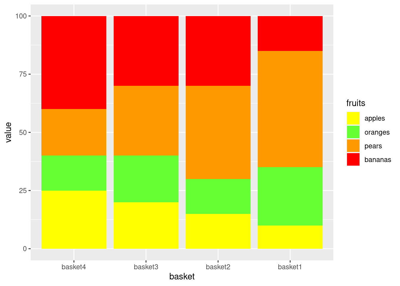

4.2.3.2 Reverse order bars according to oranges share

library(ggplot2)
df$basket <- factor(df$basket, 
                    levels=df[order(df[df$fruits == "oranges",]$value),]$basket)

ggplot(data=df[order(df$fruits),], 
       aes(x=basket,
           y=value,
           fill=fruits,
           order=fruits)) + 
  geom_bar(stat="identity", 
           position = "stack") +
  scale_fill_manual(values=fill_palette, 
                    guide = guide_legend(reverse=TRUE))

4.2.3.3 Reverse order bars according to oranges share AND place oranges at the bottom

library(ggplot2)
df$basket <- factor(df$basket, 
                    levels=df[order(df[df$fruits == "oranges",]$value),]$basket)

df$bar_order[df$fruits == "oranges"] <- 1
df$bar_order[df$fruits == "pears"]   <- 2
df$bar_order[df$fruits == "bananas"] <- 3
df$bar_order[df$fruits == "apples"]  <- 4

ggplot(data=df[order(df$bar_order),], 
       aes(x=basket,
           y=value,
           fill=fruits)) +
  geom_bar(stat="identity", 
           position = "stack") +
  scale_fill_manual(values=fill_palette, 
                    guide = guide_legend(reverse=TRUE))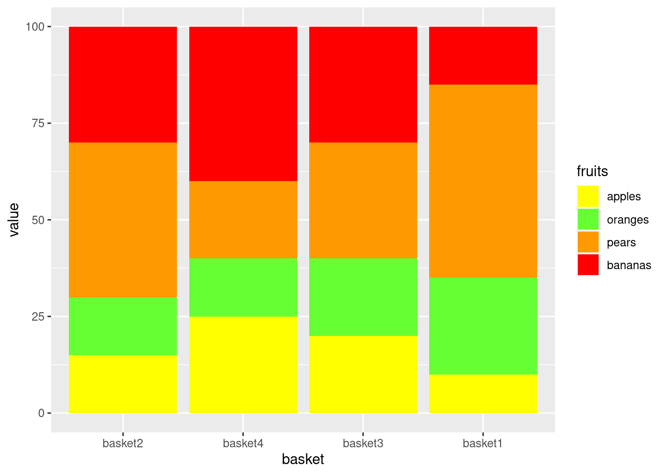

4.2.3.4 Match the colors with the fruits

library(ggplot2)

fill_palette2 <- c("#FFFF00", # yellow for bananas
                   "#66FF33", # green for pears
                   "#FF9900", # orange for orange
                   "#FF0000" # red for apple
)

ggplot(data=df[order(df$bar_order),], 
       aes(x=basket,
           y=value,
           fill=fruits)) + # This is important!!
  geom_bar(stat="identity", 
           position = "stack") +
  scale_fill_manual(values=fill_palette2)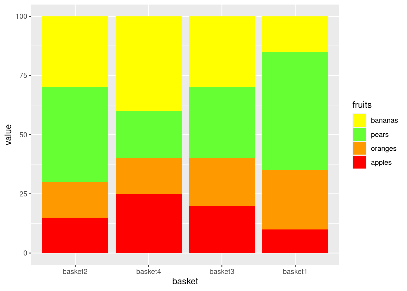

4.2.4 ….

ggplot(data=df[order(-as.numeric(df$value)),], 
       aes(x=basket,
           y=value,
           fill=fruits)) + # This is important!!
  geom_bar(stat="identity", 
           position = "stack") +
  scale_fill_manual(values=fill_palette2)

4.2.5 Links to Stack Overflow etc. on bar ordering

• How do you order the fill-colours within ggplot2 geom_bar
• ggplot legends - change labels, order and title
• ggplot2: Changing the Default Order of Legend Labels and Stacking of Data
• How do I re-arrange??: Ordering a plot revisited
• Order and color of bars in ggplot2 barplot
• Legends (ggplot2)
• how to change the order of a discrete x scale in ggplot?

---

5 Graphics using with ggplot2

5.1 Moniulotteinen hajontakuvio

library(grid)
library(ggplot2)
mtcars$brands <- row.names(mtcars)     

mtcars$am_c[mtcars$am == 0] <- "automatic"
mtcars$am_c[mtcars$am == 1] <- "manual"
mtcars$am_c <- factor(mtcars$am_c)
# keskiarvoviivat
h.lines <- data.frame(am_c=levels(mtcars$am_c), xval=c(mean(mtcars[mtcars$am_c == "automatic",]$qsec),
                                                       mean(mtcars[mtcars$am_c == "manual",]$qsec)))
v.lines <- data.frame(am_c=levels(mtcars$am_c), xval=c(mean(mtcars[mtcars$am_c == "automatic",]$mpg),
                                                       mean(mtcars[mtcars$am_c == "manual",]$mpg)))

plot <- ggplot(mtcars, aes(x=mpg,y=qsec,label=brands,color=factor(carb)))
plot <- plot + geom_point(size = 3)
plot <- plot + facet_grid(.~am_c) 
plot <- plot + geom_vline(aes(xintercept=xval), data=v.lines, linetype = "dashed", color = "grey70")
plot <- plot + geom_hline(aes(yintercept=xval), data=h.lines, linetype = "dashed", color = "grey70")
plot <- plot + geom_text(family="Open Sans", size=3.5, hjust=-.2)
plot <- plot +  labs(x="Miles/(US) gallon",
                     y="1/4 mile time")
plot <- plot + theme_minimal() + 
  theme(legend.position = "top") + 
  theme(text = element_text(family = "Open Sans", size= 12)) +
  theme(legend.title = element_text(size = 12, face = "bold")) +
  theme(axis.text= element_text(size = 10)) +
  theme(axis.title = element_text(size = 12, face = "bold")) +
  theme(legend.text= element_text(size = 12)) +
  theme(strip.text = element_text(size = 14, face="bold")) +
  guides(colour = guide_legend(override.aes = list(size=4)))  +
  theme(panel.border = element_rect(fill=NA,color="grey70", size=0.5, 
                                    linetype="solid"))
plot <- plot + coord_cartesian(xlim=c(9,40),ylim=c(15,23))
plot <- plot + scale_color_manual(values = c("#000000", "#E69F00", "#D55E00", "#009E73","#0072B2","#D55E00"))
plot <- plot + guides(color = guide_legend(title = "Number of carburetors", title.position = "top", title.hjust=.5))
plot <- plot + theme(panel.spacing = unit(2, "lines"))
plot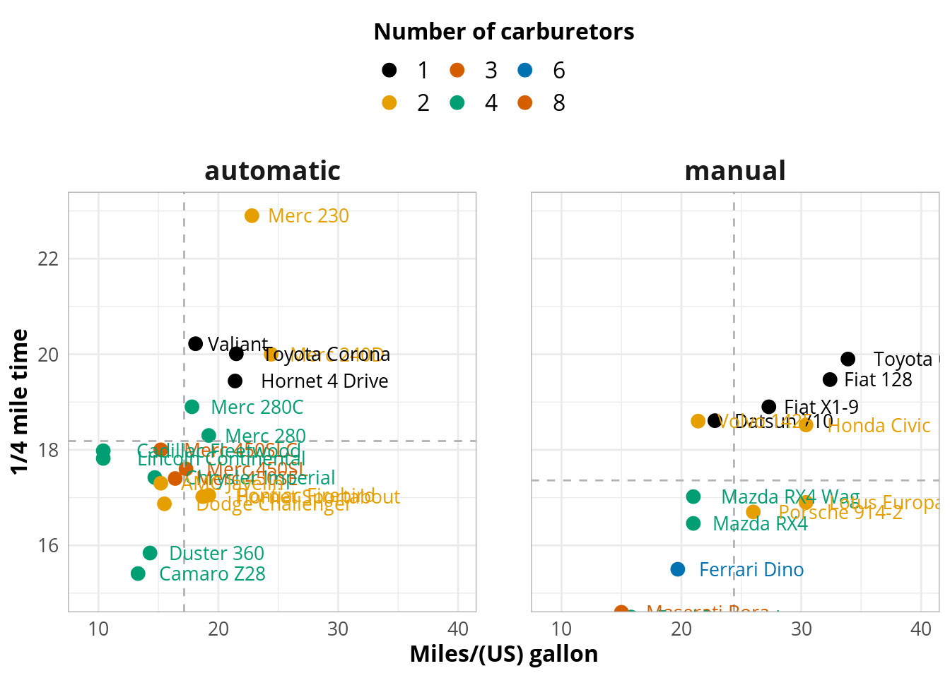

5.2 Obtaining the data and defining the colors

library(ggplot2)
library(laeken)
data(eusilc)
df <- eusilc
manual.color <- scale_color_manual(values=c("#CC79A7","#E69F00",
                                            "#56B4E9","#000000",
                                            "#009E73","#D55E00",
                                            "#0072B2","#999999",
                                            "#00FF00","Dim Grey",
                                            "#56B4E9","#000000",
                                            "#009E73","#D55E00",
                                            "#0072B2","#999999"))

manual.fill <- scale_fill_manual(values=c("#CC79A7","#E69F00",
                                          "#56B4E9","#000000",
                                          "#009E73","#D55E00",
                                          "#0072B2","#999999",
                                          "#00FF00","Dim Grey",
                                          "#56B4E9","#000000",
                                          "#009E73","#D55E00",
                                          "#0072B2","#999999"))

5.3 Bar plot

5.3.1 Proportions of female and male headed households by region

library(ggplot2)
library(grid)
tbl <- data.frame(prop.table(table(df$db040,df$rb090),1) * 100)
tbl$Freq <- round(tbl$Freq, 1)
# ordering the levels of rdb040 by femla share
df.order <- subset(tbl, Var2 == 'female')
df.order <- df.order[order(df.order$Freq),]
tbl$Var1 <- factor(tbl$Var1, levels = df.order$Var1)
# bar plot
ggplot(tbl, aes(x=Var2,y=Freq,label=Freq,fill=Var1)) +
  geom_bar(position="dodge", stat="identity") +
  geom_text(position = position_dodge(width=1), vjust=-0.5, size=3) +
  labs(x="xlab",y="ylab") +
  labs(title="plot title") +
  theme(axis.text.x  = element_text(angle=90, vjust= 0.5)) +
  coord_cartesian(ylim=c(0,75)) + 
  annotate("text", x = 1.5, y = 65, label = "Some text here") +
  theme(legend.title=element_blank()) +
  theme(legend.key.size = unit(3, "mm")) +
  theme(legend.position="top") +
  manual.fill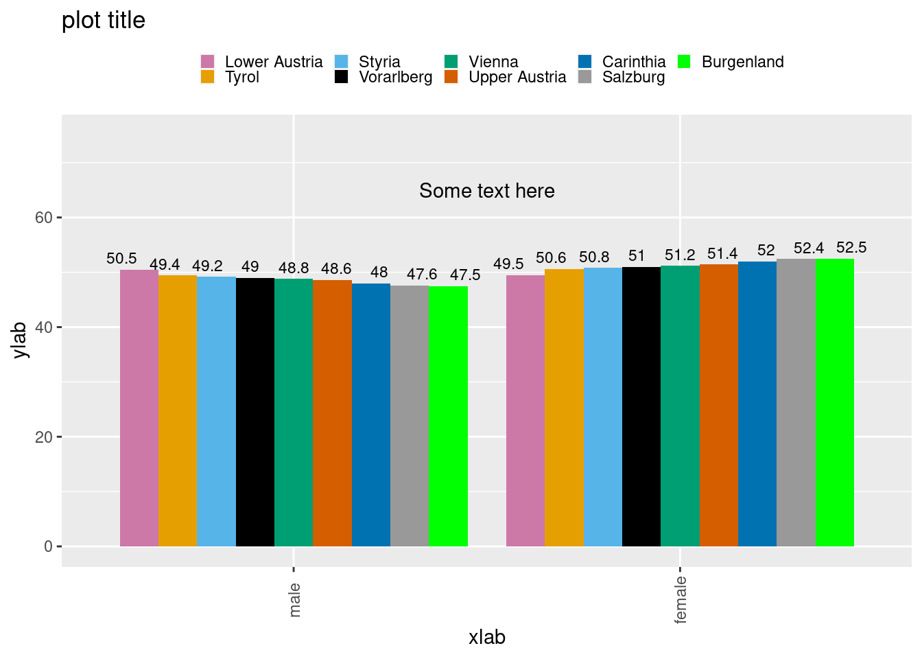

5.4 Line Plot

df <- read.csv("https://vincentarelbundock.github.io/Rdatasets/csv/Ecdat/Cigarette.csv")
df$year <- as.numeric(df$year)

cnames <- subset(df, year == 1995)
ggplot(df, 
       aes(x=year,y=packpc,group=state,color=state)) +
  geom_line() + 
  geom_point() +
  scale_x_continuous(breaks=1985:1995) +
  geom_text(data=cnames, aes(x=year,y=packpc,label=state), 
            size=4, hjust=-0.2) +
  labs(x="year",y="number of packs per capita") +
  labs(title="The Cigarette Consumption Panel Data Set") +
  theme(legend.position="none")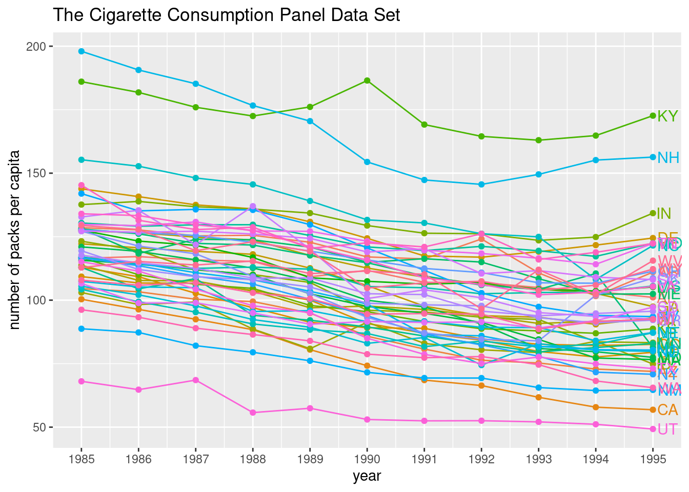

5.5 Scatter plots

5.5.1 Age vs. household income by region and sex

df <- eusilc
# aggregate a table
tbl <- aggregate(eqIncome~db040+rb090+age, 
                 median,
                 data=df)
# subset to cover ages 18-75
tbl <- subset(tbl, age > 17 & age < 76)
# plot
ggplot(tbl, aes(x=age,y=eqIncome,color=rb090)) +
  geom_point() + 
  facet_wrap(~db040) +
  geom_smooth(method=lm, se=TRUE) +
  labs(x="xlab",y="ylab") +
  labs(title="plot title") +
  theme(axis.text.x  = element_text(angle=90, vjust= 0.5)) +
  theme(legend.title=element_blank()) +
  theme(legend.key.size = unit(3, "mm")) +
  theme(legend.position="top") +
  manual.color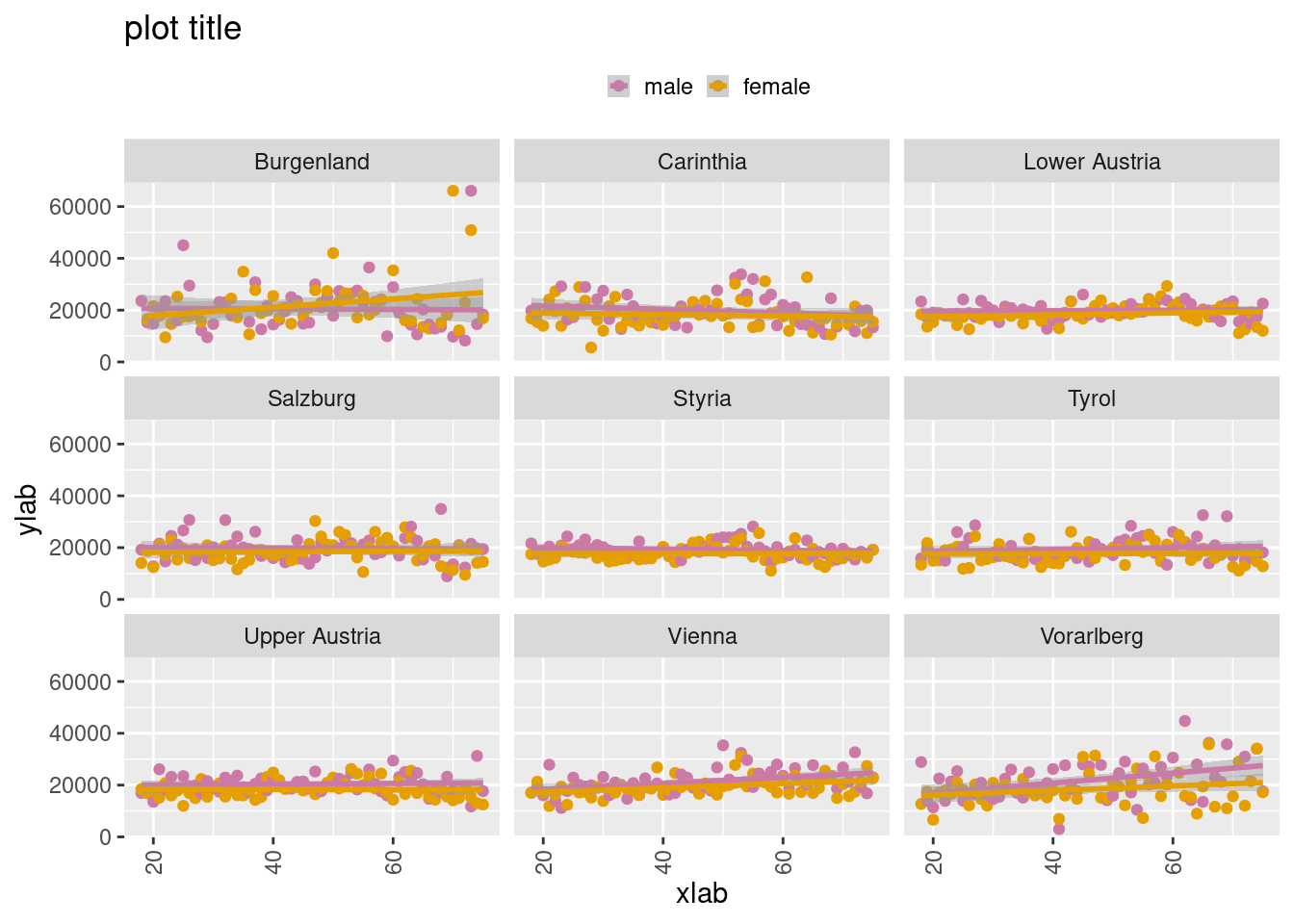

5.6 Distributions by ageclass, region and gender

5.6.1 As a density plot

df <- eusilc
df$age_class[df$age < 18] <- '0-17'
df$age_class[df$age >= 18 & df$age < 25] <- '18-24'
df$age_class[df$age >= 25 & df$age < 55] <- '26-54'
df$age_class[df$age >= 55 & df$age < 65] <- '55-64'
df$age_class[df$age >= 65] <- '65 <'

ggplot(df, aes(x=eqIncome,fill=age_class)) +
  geom_density(alpha=.4) +
  facet_grid(rb090~db040) +
  labs(x="xlab",y="ylab") +
  labs(title="plot title") +
  theme(axis.text.x  = element_text(angle=90, vjust= 0.5)) +
  theme(legend.title=element_blank()) +
  theme(legend.key.size = unit(3, "mm")) +
  theme(legend.position="top") +
  coord_cartesian(xlim=c(0,30000)) +
  manual.fill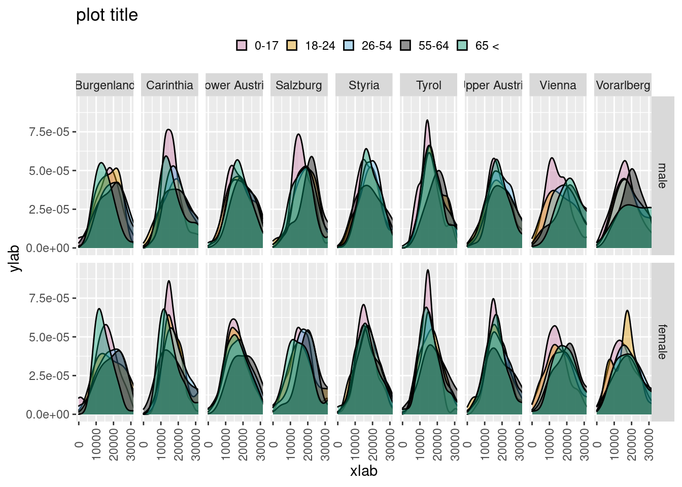

5.6.1.1 As a box plot

ggplot(df, aes(x=age_class,y=eqIncome, fill=rb090)) +
  geom_boxplot() +
  facet_wrap(~db040) +
  labs(x="xlab",y="ylab") +
  labs(title="plot title") +
  theme(axis.text.x  = element_text(angle=90, vjust= 0.5)) +
  theme(legend.title=element_blank()) +
  theme(legend.key.size = unit(3, "mm")) +
  theme(legend.position="top") +
  coord_cartesian(ylim=c(0,30000)) +
  manual.fill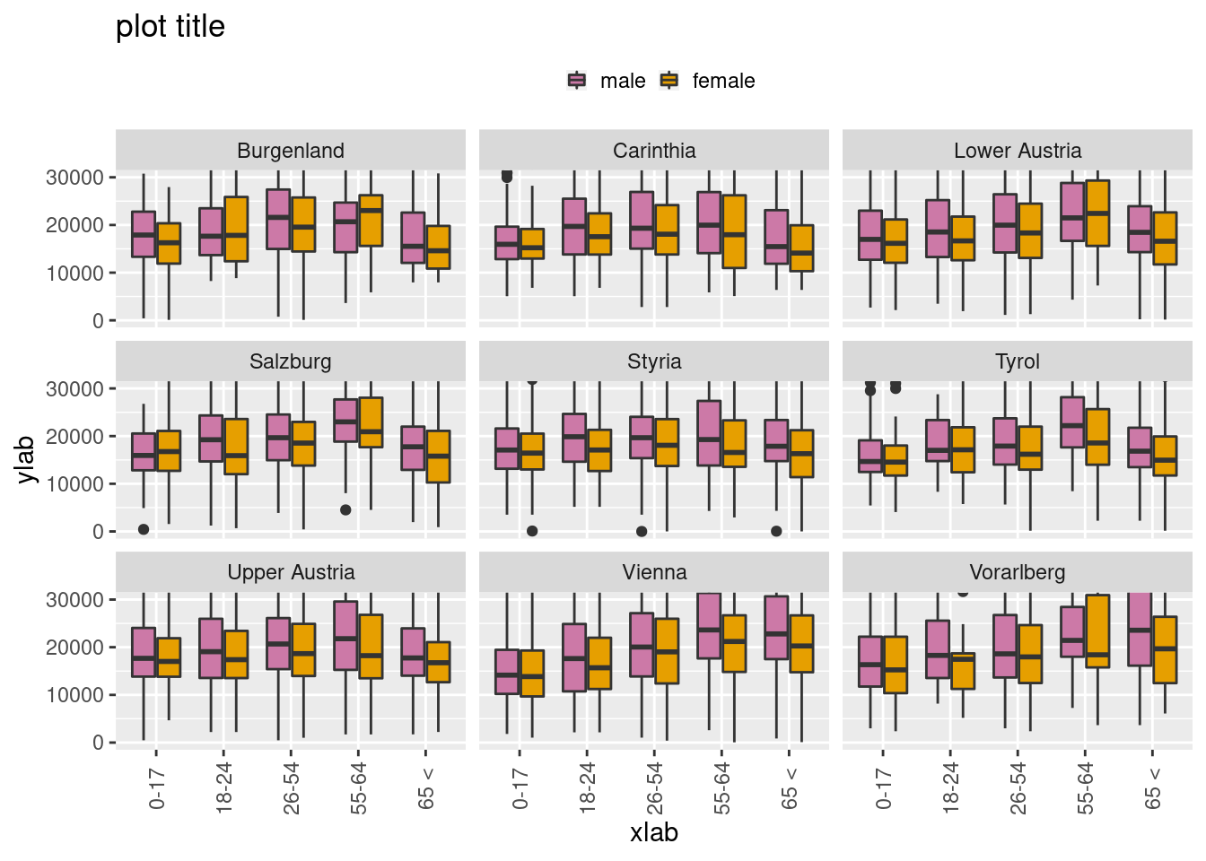

5.6.2 links

• Beautiful plotting in R: A ggplot2 cheatsheet
• Various position adjustments of legend in ggplot2

---

6 Maps with ggplot2

---

7 Survey

Resources

• survey: analysis of complex survey samples in CRAN
• Thomas Lumley: Survey analysis in R

These analysis have been made using Life in Transition Survey 2. You can load the data in R with following line of code

download.file("http://www.ebrd.com/downloads/research/surveys/lits2.dta", "lits2.dta")
lits2 <- foreign::read.dta("lits2.dta")

7.1 Survey design

library(survey)
d.df <- svydesign(id = ~SerialID, 
                  weights = ~weight, 
                  data = lits2)

7.2 Plotting distributions

dpar <- par(mfrow=c(1,2))
svyhist(~q104a_1, design=d.df, 
        main="Survey weighted",
        col="cadetblue")
lines(svysmooth(~q104a_1, d.df, bandwidth=5))
hist(lits2$q104a_1,  main="Sample unweighted",
     col="cadetblue",prob=TRUE)
lines(density(lits2$q104a_1, adjust=2))
par(dpar)

7.3 Statistical tables

7.3.1 Mean Age by country with standard errors

# Create a data.frame out of table
t <- data.frame(svyby(~q104a_1, ~q102_1+country, design=d.df, svymean, na.rm=T))
# New names for data file
names(t) <- c("Sex","Country","mean_age","SE")
# Reorder the columns
t <- t[c(2,1,3,4)]
row.names(t) <- NULL 
head(t)

##   Country Sex mean_age        SE
## 1       2   1 50.61129 0.4037583
## 2       2   2 53.90229 1.5563343
## 3       8   1 53.78624 0.5789071
## 4       8   2 57.49704 0.9782967
## 5      11   1 43.08466 0.7683500
## 6      11   2 45.63880 0.5985134

7.3.2 GRAPH with Errorbars

library(ggplot2)
ggplot(t, aes(x=Country, y=mean_age, fill=Sex)) +
  geom_bar(position="dodge", stat="identity") +
  geom_errorbar(aes(ymin=mean_age-SE, ymax=mean_age+SE), width=.2,
                position=position_dodge(.9)) +
  coord_cartesian(ylim=c(35,65)) +
  theme(axis.text.x = element_text(angle = 90, vjust = 0.5))

7.4 Quantities by categorical variable

Lets use variable q301a

The economic situation in our country is better today than around 4 years ago

# manipulate string
library(stringr)
lits2$q301a <- as.factor(str_replace(lits2$q301a, "Don't know", "Dont know"))
# recode
lits2$q301a_rec[lits2$q301a == "Strongly agree"] <- "Agree"
lits2$q301a_rec[lits2$q301a == "Agree"] <- "Agree"
lits2$q301a_rec[lits2$q301a == "Strongly disagree"] <- "Disagree"
lits2$q301a_rec[lits2$q301a == "Disagree"] <- "Disagree"
lits2$q301a_rec[lits2$q301a == "Neither disagree nor agree"] <- "Neither nor"
lits2$q301a_rec[lits2$q301a == "Dont know"] <- "Dont know"
# set levels
lits2$q301a_rec <- factor(lits2$q301a_rec, levels=c("Agree","Neither nor","Disagree","Dont know"))
######
# Re-set the survey design
d.df <- svydesign(id = ~SerialID, 
weights = ~weight, 
data = lits2)
##
t2 <- data.frame(prop.table(svytable(~q301a_rec+country, d.df),2)*100)
t2 <- t2[!is.na(t2$Freq), ]
##
ggplot(t2, aes(x=country, y=Freq, fill=q301a_rec)) + 
geom_bar(stat="identity") + 
theme(legend.position="top") + 
theme(axis.text.x = element_text(angle = 90, vjust = 0.5))

7.4.1 Share agreeing

# Freq table
## as data.frame of relative shares
t3 <- subset(t2, q301a_rec %in% 'Agree')
t3$Freq <- round(t3$Freq,1)
# plot
ggplot(t3, aes(x=reorder(country, Freq), y=Freq,label=Freq)) + 
geom_bar(stat="identity", position="dodge", fill="cadetblue") + 
coord_flip(ylim=c(0,100)) + geom_text(hjust=-0.1)

8 Värit

8.1 Color brewer

Cindy Brewer: helping you choose better color scales for maps

library(RColorBrewer)
display.brewer.all()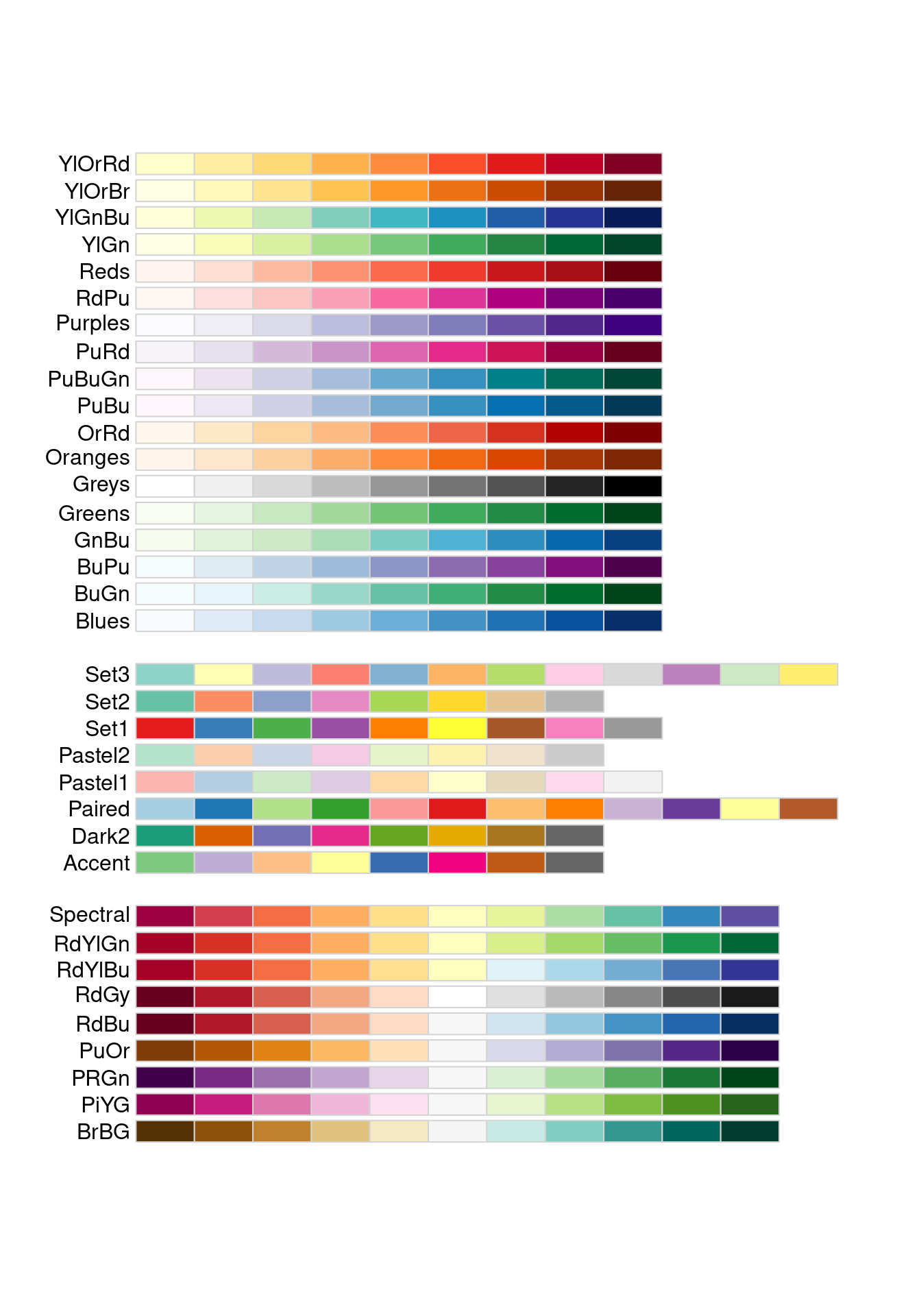

library(ggplot2)
mtcars$brands <- row.names(mtcars)     
df <- mtcars[1:10,]
plot <- ggplot(df, aes(x=brands,y=cyl,fill=factor(carb)))
plot <- plot + geom_bar(stat="identity")
plot <- plot + scale_fill_brewer(palette="Set1")
plot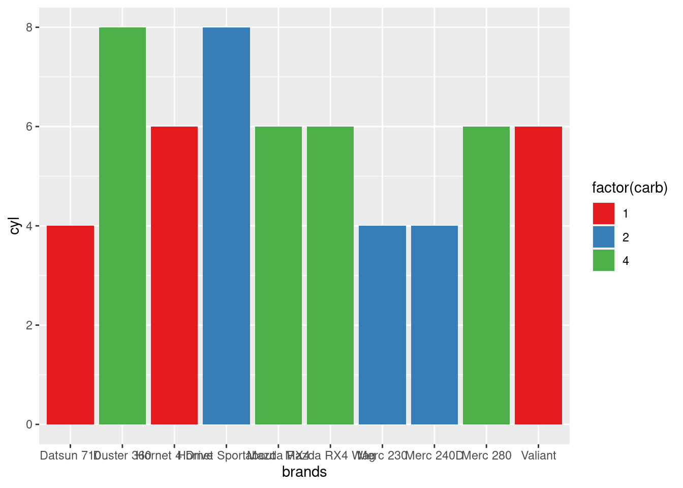

library(ggplot2)
mtcars$brands <- row.names(mtcars)     
df <- mtcars[1:8,]
plot <- ggplot(df, aes(x=hp,y=qsec,color=brands,label=brands))
plot <- plot + geom_point()
plot <- plot + geom_text(family = "Gentium", hjust=-.1)
plot <- plot + scale_color_brewer(palette="Dark2")
plot <- plot + theme(legend.position = "none")
plot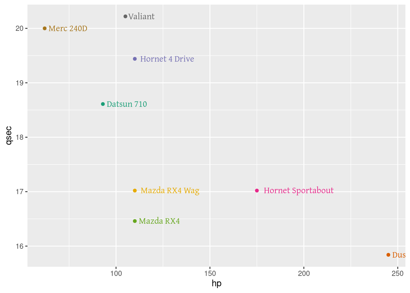

8.1.1 WesAnderson paletters

• A Wes Anderson color palette for R
• Wes Anderson Palettes.

9 Webin raapimista

9.1 Wikipedia

source

library(XML)
theurl <- "http://en.wikipedia.org/wiki/Brazil_national_football_team"
tables <- readHTMLTable(theurl)
n.rows <- unlist(lapply(tables, function(t) dim(t)[1]))

tables[[which.max(n.rows)]]

9.2 Sekalaisia

• Suomi24.fi by R-ohjelmointi.org

10 Regular expressions

10.1 Online

• https://regex101.com/

10.2 Sed

sed (stream editor) is a Unix utility that parses and transforms text, using a simple, compact programming language. sed was developed from 1973 to 1974 by Lee E. McMahon of Bell Labs,[1] and is available today for most operating systems

• http://www.grymoire.com/Unix/Sed.html
• https://www.gnu.org/software/sed/manual/sed.html

# add characters on the same line starting with "\owner"
sed -i '/^\\owner/ s/$/ }\n\\end{metadata}\n\n\\begin{metadata}{/' filex.txt

10.3 Kansanedustajien nimet

t1 <- Sys.time()
library(rvest)
library(stringr)

# generoidaan kaikkien kansanedustajien sivujen linkit
edustajat <- read_html("https://www.eduskunta.fi/FI/kansanedustajat/nykyiset_kansanedustajat/Sivut/default.aspx")
txt <- html_text(edustajat)
linkit <- unlist(stringr::str_extract_all(txt, "https://www.eduskunta.fi/FI/kansanedustajat/Sivut/[0-9]+.aspx"))

# Luodaaan tyhjä data.frame, jossa kaikki mahdolliset otsiko 
# dfs <- Filter(function(x) is(x, "data.frame"), mget(ls()))
# lapply(dfs)
# 
# nimet <- vector()
# for (nro in 1:length(dfs)){
#   nimi <- dfs[[nro]][[1]]
#   nimet <- c(nimet,nimi)
# }
# 
# uniikit_nimet <- unique(nimet)
# 
# uniikit_nimet <- gsub(":", "",uniikit_nimet)
# uniikit_nimet <- gsub("-", "",uniikit_nimet)
# uniikit_nimet <- gsub(" ", "_",uniikit_nimet)
# uniikit_nimet <- gsub(" / ", "_",uniikit_nimet)
# uniikit_nimet <- tolower(uniikit_nimet)

uniikit_nimet <- c("nimi", "puhelin", "sähköposti", "kotisivu", "ammatti_/_arvo", "vaalipiiri", 
                "toimielinjäsenyydet_ja_tehtävät", "aiemmat_toimielinjäsenyydet_ja_tehtävät", 
                "eduskuntaryhmä", "koko_nimi", "syntymäaika_ja_paikka", "kotikunta", "koulutus", 
                "työura_/_elämänkertatietoja", "vanhemmat", "puoliso", "kunnalliset_luottamustehtävät", 
                "muut_luottamustehtävät", "sotilasarvo", "toimielinjäsenyydet_ja_tehtävät_2", "nimi_2", 
                "koulutus_2", "avustaa_kansanedustajia", "puhelin_2", "sähköposti_2", "lapset", 
                "aiemmat_vaalipiirit", "aiemmat_eduskuntaryhmät", "kansanedustajana", 
                "valtiolliset_luottamustehtävät", "kansainväliset_luottamustehtävät", 
                "edustajan_julkaisut", "lisätietoja", "tehtävät_eduskuntaryhmässä", 
                "ministeri", "arvonimet", "luottamustehtävät_vallilaryhmän_yhtiöissä", 
                "muut_hallinto_ja_luottamustehtävät", "hallituksen_jäsen", "edustajantoimi_keskeytynyt", 
                "lisäksi_omistan", "pääministeri", "kouluttaja_ja_konsultti", 
                "euroa", "palkkiota_mistään_toimielimestä")

dat <- as.data.frame(setNames(replicate(length(uniikit_nimet),
                                        character(0), simplify = F), 
                              letters[1:length(uniikit_nimet)]), stringsAsFactors=FALSE)
names(dat) <- uniikit_nimet

for (linkki in linkit){
  
  edustaja <- read_html(linkki)
  cast <- html_nodes(edustaja, "#kansanedustajaMenu, .upper66")
  txt <- html_text(cast)
  d <- txt[1]
  
  d <- gsub(pattern = "\\t", replacement = "", x = d)
  d <- gsub(pattern = "\\r", replacement = "", x = d)
  # d <- gsub(pattern = "\\s\\s", replacement = "", x = d)
  
  nimi <- unlist(stringr::str_extract_all(d, "[a-öA-Ö]+\\s?([a-öA-Ö]+)?-?\\s?(\\/?|ja)\\s?([a-öA-Ö]+)?:\\n"))
  arvo <- unlist(strsplit(x = d, split = "[a-öA-Ö]+\\s?([a-öA-Ö]+)?-?\\s?(\\/?|ja)\\s?([a-öA-Ö]+)?:\\n", 
                          perl = TRUE))[-1]
  ddd <- data.frame(nimi,arvo, stringsAsFactors = FALSE)
  ddd$nimi <- stringr::str_trim(ddd$nimi) 
  ddd$nimi <- gsub(":", "",ddd$nimi)
  ddd$nimi <- gsub("-", "",ddd$nimi)
  ddd$nimi <- gsub(" ", "_",ddd$nimi)
  ddd$nimi <- gsub(" / ", "_",ddd$nimi)
  ddd$nimi <- tolower(ddd$nimi)
  # lisää duplikaatteihin
  ddd$nimi <- ifelse(duplicated(ddd$nimi),paste0(ddd$nimi,"_2"),ddd$nimi)
  ddd$arvo <- stringr::str_trim(ddd$arvo)
  ddd$arvo <- gsub("\\n", "",ddd$arvo)
  dddd <- tidyr::spread(ddd, nimi, arvo)
  dat <- bind_rows(dat,dddd)
}
duration <- Sys.time() - t1

10.4 Sosiaalidemokraattisten puolueiden kannatus Pohjoismaissa

#    __  _                           _ 
#   / _|(_)  __ _  _   _  _ __  ___ / |
#  | |_ | | / _` || | | || '__|/ _ \| |
#  |  _|| || (_| || |_| || |  |  __/| |
#  |_|  |_| \__, | \__,_||_|   \___||_|
#           |___/                      
#
#
#%#% --------------------------------------- #%#%
#%#% Scrape wikipedia 
#%#% --------------------------------------- #%#%

if (!file.exists("./local_data/df_fi.RData")){
  
  # install.packages("pxweb")
  library(pxweb)
  library(dplyr)
  library(ggplot2)
  library(ggrepel)
  library(stringr)
  library(tidyr)
  library(rvest)
  
  years <- c(1954,1958,1962,1966,1970,1972,1975,1979,1983,1987,1991,1995,1999,2003,2007,2011,2015)
  
  dd <- data.frame()
  for (y in years){
    urli <- paste0("https://fi.wikipedia.org/wiki/Eduskuntavaalit_",y)
    htmli <- read_html(urli)
    luokka <- "table.prettytable"
    if (y %in% c(1958,1979,1983,1987,1991,2011,2015)) luokka = "table.wikitable"
    n = 2
    if (y %in% c(1983,1987)) n = 3
    if (y %in% c(2007,2011,2015)) n = 1
    d <- html_table(html_nodes(htmli, luokka)[[n]], fill = T)
    d <- d[-1,]
    d <- d[c(2,5)]
    names(d) <- c("party","value")
    d <- d[ with(d, grepl("Sosialidemokraattinen Puolue", party)),]
    new_row <- data.frame(party = d$party[1],
                          value = d$value[1],
                          year = y)
    dd <- rbind(dd,new_row)
  }
  
  ddd <- dd
  dd$value <- gsub(pattern = "%", replacement = "", x= dd$value)
  dd$value <- gsub(pattern = ",", replacement = ".", x= dd$value)
  dd$value <- gsub(pattern = ",", replacement = ".", x= dd$value)
  dd$value <- str_trim(dd$value)
  dd$value <- as.factor(dd$value)
  dd$value = as.numeric(levels(dd$value))[dd$value]
  dd$party <- NULL
  dd$country <- "Finland"
  df_fi <- dd 
  save(df_fi, file="./local_data/df_fi.RData")
  
  
} else load("./local_data/df_fi.RData")


# Sweden
if (!file.exists("./local_data/df_se.RData")){
  
  library(XML)
  library(rvest)
  html <- html("https://sv.wikipedia.org/wiki/Resultat_i_val_till_Sveriges_riksdag")
  d = html_table(html_nodes(html, "table")[[1]], fill = T)
  names(d) <- d[1,]
  d <- d[-1,]
  d <- gather(d, party, value, 2:13)
  
  df_se <- d %>% filter(grepl("Social",party),
                        grepl("demokraterna",party)) %>% 
    mutate(År = as.integer(År),
            value = gsub(x=value, pattern =",", replacement = "."),
            value = as.factor(value),
            value = as.numeric(levels(value))[value]) %>% 
    filter(År >= 1950) %>% 
    rename(year = År) %>% 
    mutate(country = "Sweden") %>% 
    select(-party) 
  save(df_se, file="./local_data/df_se.RData")
  
  
} else load("./local_data/df_se.RData")


# Norway

if (!file.exists("./local_data/df_no.RData")){
  
  html <- html("https://no.wikipedia.org/wiki/Stortingsvalg_1945%E2%80%93")
  dd <- data.frame()
  tbs <- 2:18
  ys <- c(2013,2009,2005,2001,1997,1993,1989,1985,1981,1977,1973,1969,1965,1961,1957,1953,1949,1945)
  
  for (y in 1:length(tbs)){
    d = html_table(html_nodes(html, "table")[[tbs[y]]], fill = T)
    if (y != 1) d <- d[c(1,4)]
    if (y == 1) d <- d[c(2,4)]
    names(d) <- c("party","value")
    d <- d[ with(d, grepl("Arbeiderparti", party)),]
    new_row <- data.frame(party = d$party[1],
                          value = d$value[1],
                          year = ys[y])
    dd <- rbind(dd,new_row)
  }
  dd <- dd[!is.na(dd$value),]
  dd$value <- gsub(pattern = ",", replacement = ".", x= dd$value)
  dd$value <- gsub(pattern = ",", replacement = ".", x= dd$value)
  dd$value <- str_trim(dd$value)
  dd$value <- as.factor(dd$value)
  dd$value = as.numeric(levels(dd$value))[dd$value]
  dd$party <- NULL
  dd$country <- "Norway"
  df_no <- dd
  save(df_no, file="./local_data/df_no.RData")
  
} else load("./local_data/df_no.RData")



# Denmark

# https://da.wikipedia.org/wiki/Folketingsvalg#Folketingsvalg_efter_1953-grundloven

if (!file.exists("./local_data/df_dk.RData")){
  
  years <- c(1957,1960,1964,1966,1968,1971,1973,1975,1977,1979,1981,1984,1987,1988,1990,1994,1998,2001,2005,2007,2011,2015)
  
  dd <- data.frame()
  for (y in years){
    urli <- paste0("https://da.wikipedia.org/wiki/Folketingsvalget_",y)
    htmli <- read_html(urli)
    luokka <- "table.wikitable"
    if (!y %in% 2011){
      n = 1
      if (y == 2015) n = 4
      d <- html_table(html_nodes(htmli, luokka)[[n]], fill = T)
      if (!y %in% c(1984,1987,1988,1990,1994,1998,2001,2005,2007,2011,2015)) d <- d[c(1,4)]
      if (y %in% c(1984,1987,1988,1990,1994,1998,2001,2005,2007,2015)) d <- d[c(2,5)]
    } else {
      n = 3
      d <- html_table(html_nodes(htmli, luokka)[[n]], fill = T)
      d <- 
        d <- d[1:21,c(2,5)]
    }
    names(d) <- c("party","value")
    d <- d[ with(d, grepl("Socialdemok", party)),]
    new_row <- data.frame(party = d$party[1],
                          value = d$value[1],
                          year = y)
    dd <- rbind(dd,new_row)
  }
  
  ddd <- dd
  dd$value <- gsub(pattern = "%", replacement = "", x= dd$value)
  dd$value <- gsub(pattern = ",", replacement = ".", x= dd$value)
  dd$value <- gsub(pattern = ",", replacement = ".", x= dd$value)
  dd$value <- str_trim(dd$value)
  dd$value <- as.factor(dd$value)
  dd$value = as.numeric(levels(dd$value))[dd$value]
  dd$party <- NULL
  dd$country <- "Denmark"
  df_dk <- dd 
  save(df_dk, file="./local_data/df_dk.RData")
  
} else load("./local_data/df_dk.RData")



# Iceland

# http://px.hagstofa.is/pxen/pxweb/en/Ibuar/Ibuar__kosningar__althingi__althurslit/KOS02121.px

if (!file.exists("./local_data/df_ic.RData")){
  
  d <- read.csv("./local_data/KOS02121(1).csv", stringsAsFactors = FALSE, sep=";", skip = 1)
  df_ic <- d %>% filter(Category %in% "Percentage of valid votes") %>% 
    gather(., key = year, value = value, 3:17) %>% 
    mutate(year = gsub(pattern="X",replacement="",x = year),
           year = as.integer(year),
           # for value
           value = as.factor(value),
           value = as.numeric(levels(value))[value]
    ) %>% 
    filter(!is.na(value),
           grepl("Social Democratic",Political.organisation)) %>% 
    mutate(country = "Iceland") %>% 
    select(-Category,-Political.organisation)
  save(df_ic, file="./local_data/df_ic.RData")
  
} else load("./local_data/df_ic.RData")


df_nr <- rbind(df_fi,df_se,df_no,df_dk,df_ic)

#%#% --------------------------------------- #%#%
#%#% Plot
#%#% --------------------------------------- #%#%


p <- ggplot(df_nr, aes(x=year,y=value,group=country))
# disable smooth..
# p <- p + geom_smooth(aes(fill = country),method="loess", size = .5, alpha=.15, linetype="dashed") 
p <- p + geom_line(aes(color=country),size=1)
# p <- p + ggrepel::geom_text_repel(data=df_nr %>% group_by(country) %>% 
#                                     filter(year == max(year)) %>% 
#                                     mutate(value = round(value,1)) %>% 
#                                     ungroup(),
#                            aes(x=year,y=value,label=paste(country,"\n",value,"%"))
#   )
# p <- p + ggrepel::geom_text_repel(data=df_nr %>% group_by(country) %>% 
#                                     filter(year == min(year)) %>% 
#                                     mutate(value = round(value,1)) %>% 
#                                     ungroup(),
#                                   aes(x=year,y=value,label=paste(country,"\n",value,"%"))
# )
p <- p + ggrepel::geom_label_repel(data=df_nr %>% group_by(country) %>% 
                                     filter(year == max(year)) %>% 
                                     filter(country %in% c("Finland","Norway")) %>% 
                                     mutate(value = round(value,1)) %>% 
                                     ungroup(),
                                   aes(x=year,y=value,label=paste0(country,"\n",value,"%"),fill=country),
                                   lineheight=.8, alpha=.7,size=3.5,color="black",
                                   label.padding = unit(0.15, "lines"),nudge_x = 2, nudge_y=1.5
)
p <- p + ggrepel::geom_label_repel(data=df_nr %>% group_by(country) %>% 
                                     filter(year == max(year)) %>% 
                                     filter(!country %in% c("Finland","Norway")) %>% 
                                     mutate(value = round(value,1)) %>% 
                                     ungroup(),
                                   aes(x=year,y=value,label=paste0(country,"\n",value,"%"),fill=country),
                                   lineheight=.8, alpha=.7,size=3.5,color="white",
                                   label.padding = unit(0.15, "lines"),nudge_x = 2, nudge_y=-1
)

p <- p + ggrepel::geom_label_repel(data=df_nr %>% group_by(country) %>% 
                                     filter(year == min(year)) %>% 
                                     filter(country %in% c("Finland","Norway")) %>% 
                                     mutate(value = round(value,1)) %>% 
                                     ungroup(),
                                   aes(x=year,y=value,label=paste0(country,"\n",value,"%"),fill=country),
                                   lineheight=.8, alpha=.7,size=3.5,color="black",
                                   label.padding = unit(0.15, "lines"),nudge_x = 2, nudge_y=-1
)
p <- p + ggrepel::geom_label_repel(data=df_nr %>% group_by(country) %>% 
                                     filter(year == min(year)) %>% 
                                     filter(!country %in% c("Finland","Norway")) %>% 
                                     mutate(value = round(value,1)) %>% 
                                     ungroup(),
                                   aes(x=year,y=value,label=paste0(country,"\n",value,"%"),fill=country),
                                   lineheight=.8, alpha=.7,size=3.5,color="white",
                                   label.padding = unit(0.15, "lines"),nudge_x = 2, nudge_y=1
)




# VALUES AND YEARS FOR THE YEARS IN BETWEEN
# p <- p + ggrepel::geom_text_repel(data=df_nr %>% group_by(country) %>% 
#                                     filter(year != c(min(year),max(year))) %>% 
#                                     mutate(value = round(value,1)) %>% 
#                                     ungroup(),
#                                   aes(x=year,y=value,label=paste(year,"\n",value,"%")),size=2.5,alpha=.5
# )


p <- p + theme(legend.position="none")
p <- p + theme_minimal() + theme(legend.position = "none") +
  theme(text = element_text(family = fontti, size= 12)) +
  theme(legend.title = element_blank()) +
  theme(axis.text.y= element_text(size = 10)) +
  theme(axis.text.x= element_text(size = 10, angle=90, vjust= 0.5)) +
  theme(axis.title = element_text(size = 11, face = "bold")) +
  theme(legend.text= element_text(size = 11)) +
  theme(strip.text = element_text(size = 11, face = "bold")) +
  guides(colour = guide_legend(override.aes = list(size=4))) +
  theme(panel.border = element_rect(fill=NA,color="grey70", size=0.5,
                                    linetype="solid"))
# p <- p + scale_color_manual(values=c(palette_distinctive1,palette_distinctive1))
# p <- p + scale_fill_manual(values=c(palette_distinctive1,palette_distinctive1))
# p <- p + scale_fill_grey(start = .65, end = .05)
# p <- p + scale_color_grey(start = .65, end = .05)
p <- p + scale_fill_manual(values=c("black","grey80","grey30","grey60","grey10"))
p <- p + scale_color_manual(values=c("black","grey80","grey30","grey60","grey10"))
# p <- p + scale_color_manual(values=c("white","white","black","black","black"))
p <- p + scale_x_continuous(breaks = sort(unique(df_nr$year)))
p <- p + labs(x="",y="Share of votes cast in parliamentary elections (%)")

10.5 Maiden erikielisten nimien skreippaaminen wikipediasta

# load packages
library(RCurl)
library(XML)
library(stringr)

# 1. Lets parse the table of  all sovereign states from here: http://en.wikipedia.org/wiki/List_of_sovereign_states
# to get url's to English page of each state

html <- getURL("http://en.wikipedia.org/wiki/List_of_sovereign_states", followlocation = TRUE)

# parse html
doc <-  htmlParse(html, asText=TRUE)
tbls <- xpathSApply(doc, "//table[@class='sortable wikitable']", saveXML)
x <- tbls[nchar(tbls) == max(nchar(tbls))]

str <- unlist(strsplit(x, '</span><a href="/wiki/'))
str <- gsub(pattern = '\\\"(.*)', replacement = '', x = str, perl = TRUE)
str <- gsub(pattern = '\\\"(.*)', replacement = '', x = str, perl = TRUE)
str <- gsub(pattern = '(\\\n)(.*)', replacement = "", x = str, perl = TRUE)
countries <- str[-1]
# add ones not included in the list, but can be found in countrycode-package
countries <- c(countries,"Aland_Islands")

urls <- paste0("http://en.wikipedia.org/wiki/",countries)



# 2. Now we have the links, so lets go through each country page and 
# fetch the links to each language version of that page - and get there the
# language name in English AND country name in the language in question

for (i in 1:length(urls)){
  
  # download html
  html <- getURL(urls[i], followlocation = TRUE)
  
  # parse html
  doc <-  htmlParse(html, asText=TRUE)
  lists <- xpathSApply(doc, "//div[@class='body']/ul", saveXML)
  x <- lists[nchar(lists) == max(nchar(lists))]
  str <- unlist(strsplit(x, "title="))[-1]
  str <- gsub(pattern = '(\\\n)(.*)', replacement = "", x = str, perl = TRUE)
  str <- gsub(pattern = "(lang)(.*)", replacement = "", x = str, perl = TRUE)
  str <- str_replace_all(str, '\\\"','')
  
  str <- str_replace_all(str, ' – ',';')
  str <- str[grep(";", str)]
  str <- str_trim(str)
  str <- str_replace_all(str, "'","")
  
  
  ## as there are some strings with no ; marks, we get rid of them
  dd <- read.table(text = str, sep = ";", colClasses = "character")
  names(dd) <- c(countries[i],"lang")
  if (i == 1) dat <- dd
  dat <- dat[!duplicated(dat["lang"]),]
  if (i != 1) dat <- merge(dat,dd,by="lang", all.x=TRUE)
}

# finally, transpose the data

data <- as.data.frame(t(dat[-1]))

# create language names from row.names of the dat and refine them a bit
new_names <- paste0("country.name.",tolower(as.character(dat[[1]])))
new_names <- str_replace_all(new_names, " ", ".")
new_names <- str_replace_all(new_names, "/", ".")
new_names <- str_replace_all(new_names, "\\.{3}", ".")
new_names <- str_replace_all(new_names, "\\.{2}", ".")
new_names <- str_replace_all(new_names, "\\)", "")
new_names <- str_replace_all(new_names, "\\(", "")
names(data) <- new_names
# then the english country names from row.names of the data
english.name <- row.names(data)
## remove the .x's and .y's
english.name <- str_replace_all(english.name, "\\.x", "")
english.name <- str_replace_all(english.name, "\\.y", "")
## apply the new naMES
data$country.name.english <- english.name

for (i in 1:ncol(data)) {
  data[[i]] <- as.character(data[[i]])
}

# load the wiki-key data to be able to combine with original data in prep.R script
library(RCurl)
GHurl <- getURL("https://raw.githubusercontent.com/muuankarski/data/master/world/wiki_key.csv")
wiki <- read.csv(text = GHurl)
wiki[2][wiki[2] == ""] <- NA

data <- merge(data,wiki[1:2],by="country.name.english")
data <- data[c(max(ncol(data)),1:max(ncol(data))-1)]

write.csv(data, "data/wiki_names.csv", row.names = FALSE)

## Colnames to exclude in countrycode()-function
# cat(paste(shQuote(names(data), type="cmd"), collapse=", "))

11 Templates

• .Rmd

11.1 R

#' ---
#' title: 
#' author: Markus Kainu
#' date: "started Dec 28 2016 - Last updated: **`r Sys.time()`**"
#' output: 
#'   html_document:
#'     theme: yeti 
#'     toc: true
#'     toc_float: true
#'     number_sections: yes
#'     code_folding: hide
#' ---
#'
#'
#' ***
#' **Manual**
#'
#' Look [analysis.R](analysis.R) for the R-code and [plot](plot/)-folder for plots
#' 
#' Below each plot you can find links for downloading the data behind the plot in .csv format and particular plot in six different formats:
#' 
#' 1. bitmap png for screen
#' 1. pdf vector with no fonts embedded
#' 1. pdf vector with fonts embedded (using [`extrafont`](https://cran.r-project.org/web/packages/extrafont/index.html)-package)
#' 1. pdf vector with fonts included as polygons (using [`showtext`](https://cran.rstudio.com/web/packages/showtext/index.html)-package) 
#' 1. svg vector 
#' 1. svg vector with fonts included as polygons (using [`showtext`](https://cran.rstudio.com/web/packages/showtext/index.html)-package)
#'
#'  Vector formats can be edited in for example with [Inkscape](https://inkscape.org/en/) or Adobe Illustrator.
#'      
#' <b>Please email <a href="mailto:markus.kainu@gmail.com?Subject=Specify subject here" target="_top">Markus Kainu</a> 
#' for any further requirements regarding the graphs, eg. point sizes, dimensions, colors  etc.!</b>
#' 
#' ***
#' 
#+ knitr_setup, include=F
library(knitr)
knitr::opts_chunk$set(list(echo=TRUE,
                           eval=TRUE,
                           cache=FALSE,
                           warning=FALSE,
                           message=FALSE))
opts_chunk$set(fig.width = 10, fig.height = 10)

#+ setup, include=FALSE
library(stringr)
library(tidyverse)
library(extrafont)
loadfonts()
library(svglite)
library(showtext)
library(hrbrthemes)

# create folders
if (!file.exists("./plot/")) dir.create("./plot/", recursive = TRUE)
if (!file.exists("./data/")) dir.create("./data/", recursive = TRUE)
if (!file.exists("./local_data/")) dir.create("./local_data/", recursive = TRUE)

save_plot_data <- function(plot_object="p",
                           df_name = df,
                           figname = "fig1_vote_shares",
                           plot_width  = 11,
                           plot_height = 8,
                           plot_width_png = 1500,
                           plot_height_png = 1200){
  
  # Save data
  write.csv(df_name, file=paste0("./plot_csv/",figname,".csv"), row.names = F)
  # Save plot
  # png
  png(paste0("./plot/",figname,".png"), width=plot_width_png, height=plot_height_png, res = 150)
  print(get(plot_object))
  graphics.off()
  # pdf
  pdf(paste0("./plot/",figname,".pdf"), width=plot_width, height=plot_height, useDingbats = FALSE, onefile = FALSE)
  print(get(plot_object))
  graphics.off()
  # embed
  embed_fonts(file=paste0("./plot/",figname,".pdf"),
              outfile=paste0("./plot/",figname,"_emb.pdf"))
  # svg
  svglite(paste0("./plot/",figname,".svg"), width=plot_width, height=plot_height, standalone = TRUE)
  print(get(plot_object))
  graphics.off()
  # showtext pdf & svg
  showtext.auto()  ## automatically use showtext for new devices
  pdf(paste0("./plot/",figname,"_st.pdf"), width=plot_width, height=plot_height, useDingbats = FALSE, onefile = FALSE)
  print(get(plot_object))
  graphics.off()
  svglite(paste0("./plot/",figname,"_st.svg"), width=plot_width, height=plot_height, standalone = TRUE)
  print(get(plot_object))
  graphics.off()
  
  showtext.auto(FALSE)  ## turn off if no longer needed
  
}

print_download_links <- function(figname){
  
  cat(paste0(
    "![](plot/",figname,".png) \n",
    "\n",
    "- Download data in [.csv](./plot_csv/",figname,".csv) \n",
    "- Download plot in [.png](./plot/",figname,".png) \n",
    "- Download plot in [.pdf](./plot/",figname,".pdf) \n",
    "- Download plot in [.pdf](./plot/",figname,"_emb.pdf) with fonts embedded\n",
    "- Download plot in [.pdf](./plot/",figname,"_st.pdf) with fonts as shapes\n",
    "- Download plot in [.svg](./plot/",figname,".svg) \n",
    "- Download plot in [.svg](./plot/",figname,"_st.svg) with fonts as shapes\n"
  ))
}


#' 
#' # Plot1
#' 

#+ plot1
dat <- mtcars





save_plot_data(plot_object="p",
               df_name = dat1,
               figname = paste0("fig2_4t",loop_data$var[i]),
               plot_width  = 11,
               plot_height = 8,
               plot_width_png = 1650,
               plot_height_png = 1150)
print_download_links(figname = paste0("fig2_4t",loop_data$var[i]))


#'
#' ***
#' 
#' # sessioninfo()
#+ sessioninfo
sessionInfo()

12 Knitr

Knitr-asetukset

library(knitr)
opts_chunk$set(list(echo=FALSE,eval=TRUE,cache=TRUE,warning=FALSE,message=FALSE))

# tai 

library(knitr)
opts_chunk$set(list(echo=FALSE,eval=TRUE,cache=TRUE,warning=FALSE,message=FALSE,fig.height=4,dev="pdf",opts_chunk$set(fig.path = paste('figure/my-prefix-', org, sep = ''))))

12.1 Controlling plot output in html

use the following chunk settings

{r example_poland, out.width=c('300px','300px','300px','300px','300px','300px'), fig.show = "hold", fig.height=8, fig.width=6}

library(ggplot2)
resolutions <- c("60","20")
nuts_levels <- c(1,2,3)

for (res in resolutions){
  load(url(paste0("http://data.okf.fi/ropengov/avoindata/eurostat_geodata/rdata/NUTS_2013_",
                  res,
                  "M_SH.RData")))
  map.df <- get(paste0("NUTS_2013_",res,"M_SH"))
  for (lev in nuts_levels){
    m <- ggplot(data=map.df[grepl("PL", map.df$NUTS_ID) & nchar(as.character(map.df$NUTS_ID)) == lev+1,], 
                aes(x=long,y=lat,group=group)) +
      theme(title=element_text(size=20)) +
      geom_polygon(color="black",fill=NA) +
      labs(title=paste0("Poland at NUTS-",lev," level \n at 1:",res," mln resolution"))
    print(m)
  }
}

12.2 Reproducible documents with R & knitr

This summary is prepared for FAO R-user group meeting on July 1, 2015

### Resources

#### R-packages

• knitr - framework for embedding R code in markdown/latex
• rmarkdown - utilities for converting Rmarkdown/Rlatex into pdf/html/docx etc
• Sweave - the older knitr for purely latex pdf outputs

12.2.0.1 Books

• Xie, Yihui. Dynamic Documents with R and Knitr. 1 edition. Boca Raton: Chapman and Hall/CRC, 2013.
• Github-repo
• Gandrud, Christopher. Reproducible Research with R and R Studio. Boca Raton: Chapman and Hall/CRC, 2013.
• Github-repo

12.2.0.2 Quick tutorials

• R Markdown — Dynamic Documents for R
• Rmarkdown cheatsheet

12.2.0.3 Related software

• Pandoc -
• latex

12.2.1 Example 1: R-script into html/pdf

• Knitrs best hidden gem: spin
• Build a report based on an R script
• Example

script.R looks like this:

#' This is a R-script that demonstrates how to create plots and tables
#' Load the libraries first
library(knitr)
library(ggplot2)

#' Create a markdown table

kable(head(cars))

#' You can also set chunk options like this
#+ chunk-label, fig=TRUE, height=5, width=FALSE

ggplot(cars, aes(x=speed, y=dist, color=speed)) +
 geom_point() + geom_smooth(method="loess")

Use following commands for conversion in R:

knitr::spin("script.R")
# Or
rmarkdown::render("script.R")
# Or
rmarkdown::render("script.R", "html_document")

or in Rstudio simply press Crtl+Shift+k (or click the icon above the script editor)

---

Demo files are here:

• input: script.R
• pdf output: script.pdf
• html output: script.html

12.2.2 Example 2: Academic paper

Rmd. source here:

• https://raw.githubusercontent.com/muuankarski/faosyb_paper/master/faosyb_paper.Rmd

To see different formats rendered click the links from below:

• pdf: https://github.com/muuankarski/faosyb_paper/raw/master/faosyb_paper.pdf
• html: http://htmlpreview.github.io/?https://raw.githubusercontent.com/muuankarski/faosyb_paper/master/faosyb_paper.html
• Word: https://github.com/muuankarski/faosyb_paper/raw/master/faosyb_paper.docx
• Libreoffice: https://github.com/muuankarski/faosyb_paper/raw/master/faosyb_paper.odt

Templates

• pdf: https://github.com/muuankarski/faosyb_paper/blob/master/faosyb.pdf.template
• html https://github.com/muuankarski/faosyb_paper/blob/master/faosyb.html.template
• css for html: https://github.com/muuankarski/faosyb_paper/blob/master/faosyb.css

12.2.3 Example 3: Jekyll povered website

• This website
• source

12.3 Example 3:: FAO Statistical Pocketbook

• source - constantly updated
• see also wiki for documentation

12.4 Workflow

• underlaying svg

13 Pandoc

pandoc -s -S --number-section --toc --from=markdown+yaml_metadata_block -H koko_css_mukaan.css source.md -o output.html
#
pandoc -s -S --number-section --toc --from=markdown+yaml_metadata_block --css css_mukana_hakemistossa.css source.md -o output.html
# pdf
pandoc --toc --number-section --latex-engine=xelatex -V lang=english -V papersize:a4paper -V documentclass=scrartcl input.md -o article_demokr.pdf
# word
pandoc --toc --number-section input.md -o article_demokr.docx

pandoc --toc --number-section -s -S -H /home/aurelius/web/css/rmarkdown.css -r markdown+grid_tables+table_captions+yaml_metadata_block paperi-gaudeamus.md -o index.html

14 Jekyll

Start a new site

jekyll new site
cd site
jekyll serve
# => Now browse to http://localhost:4000

Asetukset ko. dokkariin

jekyll serve --watch --baseurl''

# tai

jekyll serve --watch

---

Copyright © 2016 Markus Kainu. No rights reserved.

This work is licensed under a Creative Commons Attribution 4.0 International License.